Initial Conditions
Running CMC comes in two distinct stages: generating the initial conditions, and then running CMC on those initial conditions. We briefly cover here how to create initial conditions and how to run and restart CMC.
Point-mass Initial Conditions
Generating initial conditions is the first step in running CMC. Since Version 3.4, COSMIC has been able to create CMC initial conditions, using a combination of the native binary samplers and dynamical samplers for drawing positions and velocities of clusters in virial and hydrostatic equilibrium. COSMIC can currently generate clusters from Plummer, Elson, or King profiles, as detailed below.
The examples below are also found in the examples folder of the main GitHub
repository. Note that there are two distinct options for CMC clusters:
cmc_point_mass (which we use in the Plummer and Elson examples below) will
produce a cluster of point-mass particles: no stellar radii, mass functions, or
binaries, typical for purely dynamics problems. You can see it’s options with:
In [1]: from cosmic.sample.sampler import cmc

In [2]: help(cmc.get_cmc_point_mass_sampler)
Help on function get_cmc_point_mass_sampler in module cosmic.sample.sampler.cmc:

get_cmc_point_mass_sampler(cluster_profile, size, **kwargs)
    Generates an CMC cluster model according

    Parameters
    ----------
    cluster_profile : `str`
        Model to use for the cluster profile (i.e. sampling of the placement of objects in the cluster and their velocity within the cluster)
        Options include:
        'plummer' : Standard Plummer sphere.
            Additional parameters:
            'r_max' : `float`
                the maximum radius (in virial radii) to sample the clsuter
        'elson' : EFF 1987 profile.  Generalization of Plummer that better fits young massive clusters
            Additional parameters:
            'gamma' : `float`
                steepness paramter for Elson profile; note that gamma=4 is same is Plummer
            'r_max' : `float`
                the maximum radius (in virial radii) to sample the clsuter
        'king' : King profile
            'w_0' : `float`
                King concentration parameter
            'r_max' : `float`
                the maximum radius (in virial radii) to sample the clsuter

    size : `int`
        Size of the population to sample

    Returns
    -------
    Singles: `pandas.DataFrame`
        DataFrame of Single objects in the format of the InitialCMCTable
    Binaries: `pandas.DataFrame`
        DataFrame of Single objects in the format of the InitialCMCTable
The more general cmc sampler (which we use in the King profile example
below) has all the additional features for generating stellar binaries that
COSMIC has. You can see it’s (significantly more diverse) options with
In [3]: from cosmic.sample.sampler import cmc

In [4]: help(cmc.get_cmc_sampler)
Help on function get_cmc_sampler in module cosmic.sample.sampler.cmc:

get_cmc_sampler(cluster_profile, primary_model, ecc_model, porb_model, binfrac_model, met, size, **kwargs)
    Generates an initial binary sample according to user specified models

    Parameters
    ----------
    cluster_profile : `str`
        Model to use for the cluster profile (i.e. sampling of the placement of objects in the cluster and their velocity within the cluster)
        Options include:
        'plummer' : Standard Plummer sphere.
            Additional parameters:
            'r_max' : `float`
                the maximum radius (in virial radii) to sample the clsuter
        'elson' : EFF 1987 profile.  Generalization of Plummer that better fits young massive clusters
            Additional parameters:
            'gamma' : `float`
                steepness paramter for Elson profile; note that gamma=4 is same is Plummer
            'r_max' : `float`
                the maximum radius (in virial radii) to sample the clsuter
        'king' : King profile
            'w_0' : `float`
                King concentration parameter
            'r_max' : `float`
                the maximum radius (in virial radii) to sample the clsuter

    primary_model : `str`
        Model to sample primary mass; choices include: kroupa93, kroupa01, salpeter55, custom
        if 'custom' is selected, must also pass arguemts:
        alphas : `array`
            list of power law indicies
        mcuts : `array`
            breaks in the power laws.
        e.g. alphas=[-1.3,-2.3,-2.3],mcuts=[0.08,0.5,1.0,150.] reproduces standard Kroupa2001 IMF

    ecc_model : `str`
        Model to sample eccentricity; choices include: thermal, uniform, sana12

    porb_model : `str`
        Model to sample orbital period; choices include: log_uniform, sana12

    msort : `float`
        Stars with M>msort can have different pairing and sampling of companions

    pair : `float`
        Sets the pairing of stars M>msort only with stars with M>msort

    binfrac_model : `str or float`
        Model for binary fraction; choices include: vanHaaften or a fraction where 1.0 is 100% binaries

    binfrac_model_msort : `str or float`
        Same as binfrac_model for M>msort

    qmin : `float`
        kwarg which sets the minimum mass ratio for sampling the secondary
        where the mass ratio distribution is flat in q
        if q > 0, qmin sets the minimum mass ratio
        q = -1, this limits the minimum mass ratio to be set such that
        the pre-MS lifetime of the secondary is not longer than the full
        lifetime of the primary if it were to evolve as a single star

    m2_min : `float`
        kwarg which sets the minimum secondary mass for sampling
        the secondary as uniform in mass_2 between m2_min and mass_1

    qmin_msort : `float`
        Same as qmin for M>msort; only applies if qmin is supplied

    met : `float`
        Sets the metallicity of the binary population where solar metallicity is zsun

    size : `int`
        Size of the population to sample

    zsun : `float`
        optional kwarg for setting effective radii, default is 0.02

    Optional Parameters
    -------------------
    virial_radius : `float`
        the initial virial radius of the cluster, in parsecs
        Default -- 1 pc

    tidal_radius : `float`
        the initial tidal radius of the cluster, in units of the virial_radius
        Default -- 1e6 rvir

    seed : `float`
        seed to the random number generator, for reproducability

    Returns
    -------
    Singles: `pandas.DataFrame`
        DataFrame of Single objects in the format of the InitialCMCTable

    Binaries: `pandas.DataFrame`
        DataFrame of Single objects in the format of the InitialCMCTable
Plummer Sphere
One of the most common initial conditions for a star cluster are those of Plummer (1911). They are not the most representative of star clusters in the local universe (see the King profile below), their popularity endures because their main quantities (such as enclosed mass, density, velocity dispersion, etc.) can be expressed analytically.
To generate a Plummer profile with 10,000 particles (here we only consider
point-mass particles, as opposed to real stars), we can use the following
COSMIC functions. Note that this returns two HDF5 tables, containing all the
relevant parameters for the single stars and binaries. The two tables are
linked, such
that the Singles table contains all the single stars and binary centers of mass, as well as indices pointing to the relevant binaries in Binaries.
In [5]: from cosmic.sample import InitialCMCTable

In [6]: Singles, Binaries = InitialCMCTable.sampler('cmc_point_mass', cluster_profile='plummer', size=10000, r_max=100)

In [7]: print(Singles)
           id    k       m  Reff          r        vr        vt  binind
0         1.0  0.0  0.0001   0.0   0.029964  0.483857  0.856766     0.0
1         2.0  0.0  0.0001   0.0   0.033492 -0.461177  0.664207     0.0
2         3.0  0.0  0.0001   0.0   0.034694 -0.638679  0.997434     0.0
3         4.0  0.0  0.0001   0.0   0.047434 -0.468556  0.808870     0.0
4         5.0  0.0  0.0001   0.0   0.049135 -0.601994  0.748868     0.0
...       ...  ...     ...   ...        ...       ...       ...     ...
9995   9996.0  0.0  0.0001   0.0  29.373008  0.071705  0.206904     0.0
9996   9997.0  0.0  0.0001   0.0  37.808575  0.000110  0.067377     0.0
9997   9998.0  0.0  0.0001   0.0  45.144674  0.121053  0.032027     0.0
9998   9999.0  0.0  0.0001   0.0  52.101847 -0.011594  0.122011     0.0
9999  10000.0  0.0  0.0001   0.0  61.287149  0.051053  0.064878     0.0

[10000 rows x 8 columns]
Then we can save the initial conditions to an HDF5 file (for use in CMC) with:
In [8]: InitialCMCTable.write(Singles, Binaries, filename="plummer.hdf5")
InitialCMCTable.write automatically scales the cluster to Hénon units, where
\(G = 1\), the cluster mass is \(M_{c}=1\), the cluster energy is
\(E=-0.25\), and the virial radius is \(r_v \equiv G M_c^2 / 2|U| =
1\). These are the internal code units used by CMC.
Warning
InitialCMCTable.write scales the Singles and Binaries tables in place, so if you want to make any changes to the initial conditions after writing them, you’ll have to either create copies of the tables or generate new ones.
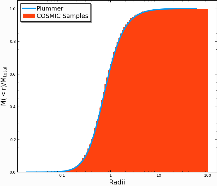
We can check that the Plummer function reproduces what we would expect from analytic predictions. The enclosed mass a Plummer sphere is given by
where \(a\) is an arbitrary scale factor (which is \(3\pi / 16\) when
the virial radius is normalized to 1). If we compare the mass-weighted
cumulative radii of our Singles Pandas table to the analytic results, we
can see:
In [9]: import numpy as np

In [10]: import matplotlib.pyplot as plt

In [11]: r_grid = np.logspace(-1.5,2,100)

In [12]: m_enc = (1 + 1/r_grid**2)**-1.5

In [13]: rv = 16/(3*np.pi) # virial radius for a Plummer sphere

In [14]: plt.plot(r_grid/rv,m_enc,lw=3);

In [15]: plt.hist(Singles.r,weights=Singles.m,cumulative=True,bins=r_grid);

In [16]: plt.xscale('log')

In [17]: plt.xlabel("Radii",fontsize=15);

In [18]: plt.ylabel(r"$M (< r) / M_{\rm total}$",fontsize=15);

In [19]: plt.legend(("Plummer","COSMIC Samples"),fontsize=14);
Elson Profile
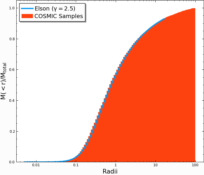
The Elson (1987) profile is a generalization of the Plummer profile that has been shown to better represent young massive clusters in the local universe. The density at a radius \(r\) is given by
Note that \(\gamma = 4\) gives a Plummer profile (the above code actually just calls the Elson profile generator with \(\gamma=4\)), though most young clusters are better fit with \(\gamma\sim2-3\). The enclosed mass is correspondingly more complicated:
Where \(\,_2F_1\) is the ordinary hypergeometric function.
Unlike both the Plummer and King profiles, the distribution function for the Elson profile cannot be written analytically. To generate the initial conditions, we directly integrate the density and potential functions to numerically compute \(f(E)\), and draw our velocity samples from that (see appendix B of Grudic et al., 2018). This produces a handful of warnings in the SciPy integrators, but the profiles that it generates are correct.
To generate an Elson profile with \(\gamma=2.5\), we can use
In [20]: Singles, Binaries = InitialCMCTable.sampler('cmc_point_mass', cluster_profile='elson', gamma=2.5, size=10000, r_max=100)
Comparing with the theoretical calculation for the enclosed mass, we find similarly good agreement:
In [21]: from scipy.special import hyp2f1

In [22]: gamma = 2.5

In [23]: def m_enc(gamma,r,rho_0):
   ....:     return 4*np.pi*rho_0/3 * r**3 * hyp2f1(1.5,(gamma+1)/2,2.5,-r**2)
   ....:

In [24]: rv = 6. ## virial radius for a gamma=2.5 Elson profile

In [25]: rho_0 = 1/m_enc(gamma,100*rv,1)

In [26]: plt.plot(r_grid/rv,m_enc(gamma,r_grid,rho_0),lw=3); # note we scale by rv, rather than set scale factor

In [27]: plt.hist(Singles.r,weights=Singles.m,cumulative=True,bins=r_grid);

In [28]: plt.xscale('log')

In [29]: plt.xlabel("Radii",fontsize=15);

In [30]: plt.ylabel(r"$M (< r) / M_{\rm total}$",fontsize=15);

In [31]: plt.legend(("Elson ($\gamma=2.5$)","COSMIC Samples"),fontsize=14);
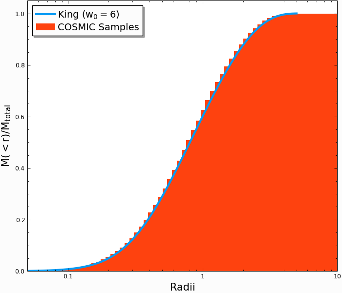
King Profile
An idealized cluster in thermodynamic equilibrium could be described as an isothermal sphere, where the velocities of stars resembled a Maxwell-Boltzmann distribution. But the isothermal sphere has infinite mass, and in any realistic star cluster, the distribution of stars should go to zero near the tidal boundary. The King (1966) profile accomplishes this by sampling from a lowered isothermal distribution
The King initial conditions can be created with COSMIC using:
In [32]: Singles, Binaries = InitialCMCTable.sampler('cmc_point_mass', cluster_profile='king', w_0=6, size=10000, r_max=100)
The analytic form of \(M(<r)\) cannot be written down for a King profile, but we can solve the ODE directly (this is done when generating the samples)
In [33]: from cosmic.sample.cmc import king

In [34]: radii,rho,phi,m_enc = king.integrate_king_profile(6)

In [35]: rho /= m_enc[-1]

In [36]: m_enc /= m_enc[-1]

In [37]: rv = king.virial_radius_numerical(radii, rho, m_enc) # just compute R_v numerically

In [38]: plt.plot(radii/rv,m_enc,lw=3);

In [39]: plt.hist(Singles.r,weights=Singles.m,cumulative=True,bins=r_grid);

In [40]: plt.xscale('log')

In [41]: plt.xlim(0.05,10);

In [42]: plt.xlabel("Radii",fontsize=15);

In [43]: plt.ylabel(r"$M (< r) / M_{\rm total}$",fontsize=15);

In [44]: plt.legend(("King ($w_0=6$)","COSMIC Samples"),fontsize=14);
Realistic Initial Conditions
So far the above examples have only used the cmc_point_mass sampler. To
generate realistic initial conditions, with stellar masses and binaries, we
want to use the cmc sampler instead. This enables all the additional
options found in the independent population sampler that COSMIC uses (see
here for more details).
To generate the above King profile, but with all the additional stellar physics (initial mass function, binaries, etc.) we would use
In [45]: Singles, Binaries = InitialCMCTable.sampler('cmc', binfrac_model=0.1, primary_model='kroupa01',
   ....:                                             ecc_model='thermal', porb_model='log_uniform', qmin=0.1, m2_min=0.08,
   ....:                                             cluster_profile='king', met=0.00017, zsun=0.017, size=100000,w_0=6,
   ....:                                             seed=12345,virial_radius=1,tidal_radius=1e6)
   ....:
This example is also found in the examples folder in the CMC repository.
Warning
At this step the metallicity (met) and value of the solar metallicity (zsun) must be specified to generate the correct initial radii for stars. If you have a very compact cluster and the value of zsun differs between here and your ini file, you may produce binaries which merge during cluster initialization, which breaks the code.
